MNIST Digit Classifier in TensorFlow
I’m currently progressing through the Advanced Learning Algorithms course by Andrew Ng. To get some hands-on practice, I decided to work on the classic MNIST dataset, which contains 60,000 28×28 grayscale images of handwritten digits (0 to 9). The dataset can be downloaded directly from the MNIST homepage.
Jupyter Notebook
To get started, I used a Jupyter Notebook running TensorFlow, installed via my Kubeflow on K8s.

Load Data
TensorFlow provides a convenient way to load the MNIST dataset.
import tensorflow as tf
from tensorflow import keras

(X_train, y_train), (X_test, y_test) = keras.datasets.mnist.load_data()
assert X_train.shape == (60000, 28, 28)
assert X_test.shape == (10000, 28, 28)
assert y_train.shape == (60000,)
assert y_test.shape == (10000,)
Visualise the Data
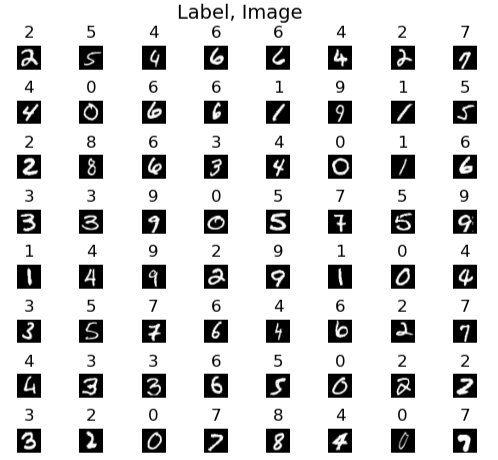
To better understand the dataset, I visualized a random sample of 64 digits from the training set:
import numpy as np
import matplotlib.pyplot as plt
import warnings

warnings.simplefilter(action='ignore', category=FutureWarning)

m = X_train.shape[0]

fig, axes = plt.subplots(8, 8, figsize=(5, 5))
fig.tight_layout(pad=0.13, rect=[0, 0.03, 1, 0.91])

for i, ax in enumerate(axes.flat):
    random_index = np.random.randint(m)
    image_to_display = X_train[random_index].reshape((28, 28))
    ax.imshow(image_to_display, cmap='gray')
    ax.set_title(y_train[random_index])
    ax.set_axis_off()

fig.suptitle("Label, Image", fontsize=14)
plt.show()
Model Representation
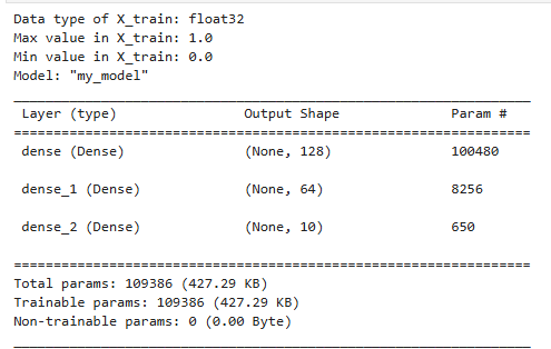
Each image is a 28×28 pixel grid, which we “unroll” into a 784-dimensional input vector. The architecture of our neural network is:
- Input layer: 784 units
- Hidden layer 1: 128 units (ReLU)
- Hidden layer 2: 64 units (ReLU)
- Output layer: 10 units (for digits 0–9)
We start by normalizing pixel values from 0–255 to 0–1 and flattening the image data:
from tensorflow.keras.models import Sequential
from tensorflow.keras.layers import Dense
from tensorflow.keras.activations import linear, relu

X_train = X_train.astype('float32') / 255.0
X_test = X_test.astype('float32') / 255.0

X_train = X_train.reshape(X_train.shape[0], -1)
X_test = X_test.reshape(X_test.shape[0], -1)

tf.random.set_seed(1234)
model = Sequential([
        Dense(128, activation='relu', input_shape=(784,)),
        Dense(64, activation='relu'),
        Dense(10, activation='linear')
], name = "my_model")

model.compile(
    loss=tf.keras.losses.SparseCategoricalCrossentropy(from_logits=True),
    optimizer=tf.keras.optimizers.Adam(0.001),
    metrics=['accuracy']
)

model.summary()
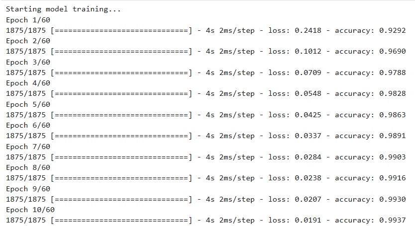
Train the Model
print("Starting model training...")
history = model.fit(
    X_train,
    y_train,
    epochs=60
)
print("Model training finished.")
Evaluate the Model
print("\nEvaluating model on test data...")
loss, accuracy = model.evaluate(X_test, y_test, verbose=0)
print(f"Test Loss: {loss:.4f}")
print(f"Test Accuracy: {accuracy:.4f}")
# Sample output
Evaluating model on test data...
Test Loss: 0.1928
Test Accuracy: 0.9815
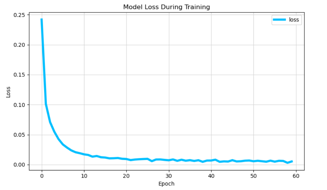
Loss (Cost) Plot
def plot_loss_tf(history):
    try:
        fig, ax = plt.subplots(figsize=(8, 5))
        ax.plot(history.history['loss'], label='loss', color='deepskyblue', linewidth=4)
        ax.set_title('Model Loss During Training')
        ax.set_ylabel('Loss')
        ax.set_xlabel('Epoch')
        ax.legend(loc='upper right')
        ax.grid(True, color='lightgrey', linestyle='-')

        plt.tight_layout()
        plt.show()
    except Exception as e:
        print(f"Error plotting: {e}")

plot_loss_tf(history)
Model Prediction
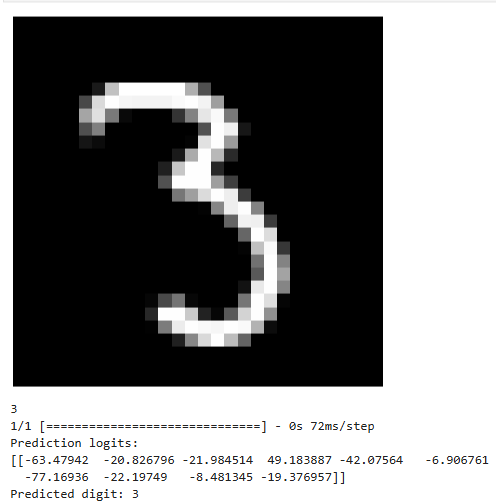
Let’s try predicting a digit:
import numpy as np

def display_digit(image_vector):
    try:
        image_matrix = image_vector.reshape((28, 28))
    except ValueError as e:
        print(f"Error reshaping vector of size {num_pixels} to {dimension}x{dimension}: {e}")
        return

    plt.imshow(image_matrix, cmap='gray')
    plt.axis('off')
    plt.show()

image_of_three = X_train[8888]
display_digit(image_of_three)
print(y_train[8888])

prediction = model.predict(image_of_three.reshape(1,784))
print(f"Prediction logits:\n{prediction}")
print(f"Predicted digit: {np.argmax(prediction)}")
Convert Logits to Probabilities
prediction_p = tf.nn.softmax(prediction)
print(f"Probability vector:\n{prediction_p}")
print(f"Sum of probabilities: {np.sum(prediction_p):.3f}")
# Sample output
Probability vector:
Probability vector:
[[1.1407684e-31 3.7281105e-25 1.1554550e-28 1.0000000e+00 4.0587488e-31
  4.0818696e-23 0.0000000e+00 1.4413385e-26 1.2729607e-21 7.6773376e-23]]
Sum of probabilities: 1.000
Index of the largest probability for predicted target
yhat = np.argmax(prediction_p)
print(f"np.argmax(prediction_p): {yhat}")
# Sample output
np.argmax(prediction_p): 3
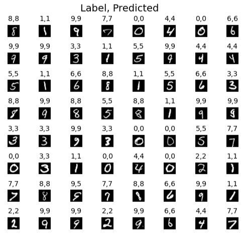
Prediction on Sample Set
fig, axes = plt.subplots(8,8, figsize=(5,5))
fig.tight_layout(pad=0.13,rect=[0, 0.03, 1, 0.91])

for i,ax in enumerate(axes.flat):
    random_index = np.random.randint(m)
    image = X_train[random_index].reshape((28,28))
    prediction = model.predict(X_train[random_index].reshape(1,-1), verbose=0)
    yhat = np.argmax(tf.nn.softmax(prediction))

    ax.imshow(image, cmap='gray')
    ax.set_title(f"{y_train[random_index]},{yhat}", fontsize=10)
    ax.set_axis_off()

fig.suptitle("Label, Predicted", fontsize=14)
plt.show()
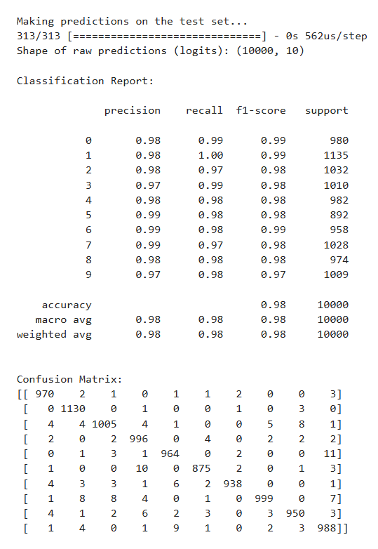
Final Evaluation on Test Set
from sklearn.metrics import classification_report, confusion_matrix

print("\nMaking predictions on the test set...")
test_logits = model.predict(X_test, verbose=1)
print("Shape of raw predictions (logits):", test_logits.shape)

test_probabilities = tf.nn.softmax(test_logits).numpy()
y_hat = np.argmax(test_probabilities, axis=1)

print("\nClassification Report:\n")
print(classification_report(y_test, y_hat))

print("\nConfusion Matrix:")
cm = confusion_matrix(y_test, y_hat)
print(cm)
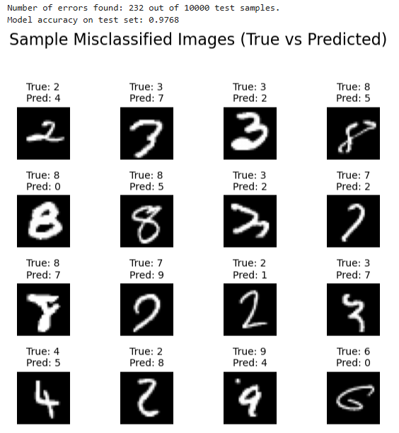
Inspect Prediction Error
error_mask = (y_hat != y_test)
error_indices = np.where(error_mask)[0]

print(f"Number of errors found: {len(error_indices)} out of {len(y_test)} test samples.")
print(f"Model accuracy on test set: {1 - (len(error_indices) / len(y_test)):.4f}")

num_errors_to_show = 16
if len(error_indices) == 0:
    print("No errors found! Model is perfect on the test set.")
elif len(error_indices) < num_errors_to_show:
    print(f"Warning: Found only {len(error_indices)} errors, displaying all of them.")
    selected_error_indices = error_indices
    num_errors_to_show = len(error_indices)
else:
    selected_error_indices = np.random.choice(error_indices, num_errors_to_show, replace=False)

if num_errors_to_show > 0:
    grid_size = int(np.ceil(np.sqrt(num_errors_to_show)))

    fig, axes = plt.subplots(grid_size, grid_size, figsize=(6, 6))
    fig.suptitle(f'Sample Misclassified Images (True vs Predicted)', fontsize=16)

    axes_flat = axes.flatten()
    for i, error_idx in enumerate(selected_error_indices):
        ax = axes_flat[i]

        image_vector = X_test[error_idx]
        image_to_display = image_vector.reshape((28, 28))
        true_label = y_test[error_idx]
        predicted_label = y_hat[error_idx]

        ax.imshow(image_to_display, cmap='gray')
        ax.set_title(f"True: {true_label}\nPred: {predicted_label}", fontsize=10)
        ax.set_axis_off()

    for j in range(i + 1, len(axes_flat)):
         axes_flat[j].set_visible(False)

    plt.tight_layout(rect=[0, 0.03, 1, 0.95])
    plt.show()
Conclusion
This was a great hands-on experience to reinforce the theory from Andrew Ng’s course. The model achieved over 97% accuracy on the test set using a simple feedforward neural network. Moving forward, I’m keen to explore more varied model architectures to further improve performance.